Understanding the Stan codebase - Part 2: Samplers

Introduction

Recap of Part 1

We pick up from where we left off in Part 1. We found out that CmdStan calls the Stan services in cmdstan::command(). For example with the command-line call

mymodel.exe id=1 method=sample algorithm=hmc engine=nuts adapt engaged=1

1. the called service is stan::services::sample::hmc_nuts_diag_e_adapt()
2. which then calls stan::services::util::run_adaptive_sampler()
3. which calls stan::services::util::generate_transitions().

Note: All code pieces shown from now on in this post are adapted from https://github.com/stan-dev/stan, licenced under the new BSD licence. Comments starting with ... indicate parts of source code that have been left out from original source code. During writing of this post, the most recent Stan version is 2.28.2. The hyperlinks to source code cannot be guaranteed to work in the future, if the source repo organization is changed or files are renamed.

Starting point for Part 2

We find generate_transitions() in generate_transitions.hpp.

void generate_transitions(stan::mcmc::base_mcmc& sampler, int num_iterations,
                          ..., stan::mcmc::sample& init_s, Model& model, ...) {
  for (int m = 0; m < num_iterations; ++m) {
    // ... callbacks and progress printing
    init_s = sampler.transition(init_s, logger);
    // ... writing to output
  }
}

Among other things, it takes as input the sampler, model, and initial point in parameter space. The function is basically just a loop that calls sampler.transition() repeatedly for num_iterations times. Therefore all interesting algorithmic code and properties that define how sampling works, whether adaptation is performed etc, have to be included as part of sampler.

This is why we now jump from the stan::services namespace to stan::mcmc, where the different samplers and their transitions are defined.

Samplers

We see in generate_transitions() that sampler has to have type base_mcmc. However, in stan::services::sample::hmc_nuts_diag_e_adapt(), our sampler was declared as

stan::mcmc::adapt_diag_e_nuts<Model, boost::ecuyer1988> sampler(model, rng);

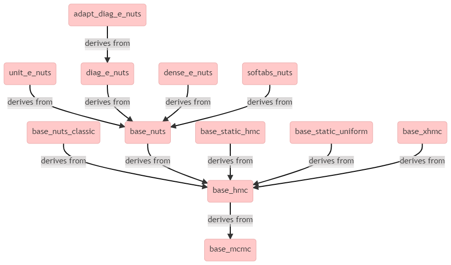
It appears that adapt_diag_e_nuts is a (templated) class that derives from base_mcmc through multiple levels of inheritance as can be seen from the above diagram.

base_mcmc

This is just an interface for all MCMC samplers, as it doesn’t contain any function bodies.

class base_mcmc {
 public:
  base_mcmc() {}

  virtual ~base_mcmc() {}

  virtual sample transition(sample& init_sample, callbacks::logger& logger) = 0;

  virtual void get_sampler_param_names(std::vector<std::string>& names) {}

  virtual void get_sampler_params(std::vector<double>& values) {}

  //... other virtual functions without body

};

The class member functions are all virtual (except the constructor), meaning that deriving classes can override them. We see that transition() is pure virtual (declared with = 0), meaning that a deriving class must override it in order to be instantiable.

base_hmc

This is a base for all Hamiltonian samplers, and derives from base_mcmc.

template <class Model, template <class, class> class Hamiltonian,
          template <class> class Integrator, class BaseRNG>
class base_hmc : public base_mcmc {
 public:
  base_hmc(const Model& model, BaseRNG& rng)
      : base_mcmc(),
        z_(model.num_params_r()),
        integrator_(),
        hamiltonian_(model),
        rand_int_(rng),
        rand_uniform_(rand_int_),
        nom_epsilon_(0.1),
        epsilon_(nom_epsilon_),
        epsilon_jitter_(0.0) {}

  // ... methods defined here

 protected:
  typename Hamiltonian<Model, BaseRNG>::PointType z_;
  Integrator<Hamiltonian<Model, BaseRNG> > integrator_;
  Hamiltonian<Model, BaseRNG> hamiltonian_;

  BaseRNG& rand_int_;

  // Uniform(0, 1) RNG
  boost::uniform_01<BaseRNG&> rand_uniform_;

  double nom_epsilon_;
  double epsilon_;
  double epsilon_jitter_;
};

We see that the class doesn’t implement transition(), so it is also an abstract class. What it does do is it defines some attributes that all Hamiltonian samplers need.

class attributes

The attributes listed as protected describe the internal state of the sampler. All Hamiltonian samplers have these attributes, and the most intersting ones of them are

• z_: current state of the sampler (point in parameter space)
• integrator_: numerical integrator used to simulate the Hamiltonian dynamics
• hamiltonian_: the Hamiltonian system
• epsilon_ / nom_epsilon_: step size of the integrator

getters

The above are private attributes and should not be directly accessed from outside. Instead, there are some getter methods that can be used, for example

  typename Hamiltonian<Model, BaseRNG>::PointType& z() { return z_; }

init_stepsize()

The first actual algorithm that we encouter is the init_stepsize() method of the base_hmc class, defined in base_hmc.hpp. This defines how the integrator’s initial stepsize (possibly given by user) is refined. As we saw in Part 1, this gets called in stan::services::sample::hmc_nuts_diag_e_adapt() before any MCMC iterations are done.

  void init_stepsize(callbacks::logger& logger) {
    ps_point z_init(this->z_);

    // Skip initialization for extreme step sizes
    if (this->nom_epsilon_ == 0 || this->nom_epsilon_ > 1e7
        || std::isnan(this->nom_epsilon_))
      return;

    this->hamiltonian_.sample_p(this->z_, this->rand_int_);
    this->hamiltonian_.init(this->z_, logger);

    // Guaranteed to be finite if randomly initialized
    double H0 = this->hamiltonian_.H(this->z_);

    this->integrator_.evolve(this->z_, this->hamiltonian_, this->nom_epsilon_,
                             logger);

    double h = this->hamiltonian_.H(this->z_);
    if (std::isnan(h))
      h = std::numeric_limits<double>::infinity();

    double delta_H = H0 - h;

    int direction = delta_H > std::log(0.8) ? 1 : -1;

    while (1) {
      this->z_.ps_point::operator=(z_init);

      this->hamiltonian_.sample_p(this->z_, this->rand_int_);
      this->hamiltonian_.init(this->z_, logger);

      double H0 = this->hamiltonian_.H(this->z_);

      this->integrator_.evolve(this->z_, this->hamiltonian_, this->nom_epsilon_,
                               logger);

      double h = this->hamiltonian_.H(this->z_);
      if (std::isnan(h))
        h = std::numeric_limits<double>::infinity();

      double delta_H = H0 - h;

      if ((direction == 1) && !(delta_H > std::log(0.8)))
        break;
      else if ((direction == -1) && !(delta_H < std::log(0.8)))
        break;
      else
        this->nom_epsilon_ = direction == 1 ? 2.0 * this->nom_epsilon_
                                            : 0.5 * this->nom_epsilon_;

      if (this->nom_epsilon_ > 1e7)
        throw std::runtime_error(
            "Posterior is improper. "
            "Please check your model.");
      if (this->nom_epsilon_ == 0)
        throw std::runtime_error(
            "No acceptably small step size could "
            "be found. Perhaps the posterior is "
            "not continuous?");
    }

    this->z_.ps_point::operator=(z_init);
  }

On the lines

    double H0 = this->hamiltonian_.H(this->z_);
    this->integrator_.evolve(this->z_, this->hamiltonian_, this->nom_epsilon_,logger);
    double h = this->hamiltonian_.H(this->z_);
    double delta_H = H0 - h;

the Hamiltonian is first computed at the current point z_, then the integrator evolves the state, after which the Hamiltonian is computed at the new state. The change in Hamiltonian (delta_H) then determines how the nominal stepsize (nom_epsilon_) is refined, or if it is suitable so that the actual MCMC sampling can start.

base_nuts

This is defined in base_nuts.hpp, and is the base class for No-U-Turn samplers with multinomial sampling. This class, which derives from base_hmc, is the first place where we encounter an implementation of transition(). You can read the comments in the source code of the transition() method to get and idea of the progress of the algorithm. We won’t go into details of the NUTS algorithm here, but just notice that the transition() function takes as input a sample& init_sample and generates a new sample object and returns it. Here, sample is a class that describes one MCMC draw, and it is defined in sample.hpp.

diag_e_nuts

This is a base class for NUTS with the diagonal HMC metric (diagonal mass matrix), and derives from base_nuts. There are similar classes for the dense and unit metric too. There are no new methods here.

adapt_diag_e_nuts

Finally we get to the class the defines the adaptive NUTS sampler with the diagnal metric. This class, adapt_diag_e_nuts, derives from diag_e_nuts. It overrides the transition() method with

  sample transition(sample& init_sample, callbacks::logger& logger) {
    sample s = diag_e_nuts<Model, BaseRNG>::transition(init_sample, logger);

    if (this->adapt_flag_) {
      this->stepsize_adaptation_.learn_stepsize(this->nom_epsilon_,
                                                s.accept_stat());

      bool update = this->var_adaptation_.learn_variance(this->z_.inv_e_metric_,
                                                         this->z_.q);

      if (update) {
        this->init_stepsize(logger);

        this->stepsize_adaptation_.set_mu(log(10 * this->nom_epsilon_));
        this->stepsize_adaptation_.restart();
      }
    }
    return s;
  }

The actual transition

sample s = diag_e_nuts<Model, BaseRNG>::transition(init_sample, logger);

The other code is for adapting the HMC metric and the integrator step size. To study how this work, we need to find out what stepsize_adaptation_ and var_adaptation_ are. However, we can’t seem to find them in adapt_diag_e_nuts.hpp. So what is again going on?

Adaptation

We find that in addition to diag_e_nuts, the adapt_diag_e_nuts class derives also from another class, called stepsize_var_adapter (defined in stepsize_var_adapter.hpp).

Class hierarchy

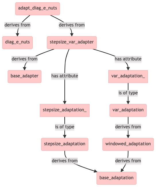
The above diagram explains why sampler objects of class adapt_diag_e_nuts have the stepsize_adaptation_ and var_adaptation_ attributes. The former is for adapting the integrator step size and the latter for adapting the mass matrix diagonal. The metric is adapted in three windows, which are called init_buffer, term_buffer and base_window. The the most abstract base class is base_adaptation, which doesn’t contain any implemented methods.

Algorithms

Let’s now return to studying the transition() method of the adapt_diag_e_nuts class. When the adapt_flag_ is on (that is, in the warmup phase), each transition will run the code

  this->stepsize_adaptation_.learn_stepsize(this->nom_epsilon_,
                                                s.accept_stat());

  bool update = this->var_adaptation_.learn_variance(this->z_.inv_e_metric_,
                                                         this->z_.q);

  if (update) {
    this->init_stepsize(logger);

    this->stepsize_adaptation_.set_mu(log(10 * this->nom_epsilon_));
    this->stepsize_adaptation_.restart();
  }

learn_stepsize()

The learn_stepsize() algorithm is defined in stepsize_adaptation.hpp.

void learn_stepsize(double& epsilon, double adapt_stat) {
    ++counter_;

    adapt_stat = adapt_stat > 1 ? 1 : adapt_stat;

    // Nesterov Dual-Averaging of log(epsilon)
    const double eta = 1.0 / (counter_ + t0_);

    s_bar_ = (1.0 - eta) * s_bar_ + eta * (delta_ - adapt_stat);

    const double x = mu_ - s_bar_ * std::sqrt(counter_) / gamma_;
    const double x_eta = std::pow(counter_, -kappa_);

    x_bar_ = (1.0 - x_eta) * x_bar_ + x_eta * x;

    epsilon = std::exp(x);
  }

learn_variance()

The learn_variance() algorithm on the otherhand is defined in var_adaptation.hpp

bool learn_variance(Eigen::VectorXd& var, const Eigen::VectorXd& q) {
    if (adaptation_window())
      estimator_.add_sample(q);

    if (end_adaptation_window()) {
      compute_next_window();

      estimator_.sample_variance(var);

      double n = static_cast<double>(estimator_.num_samples());
      var = (n / (n + 5.0)) * var
            + 1e-3 * (5.0 / (n + 5.0)) * Eigen::VectorXd::Ones(var.size());

      if (!var.allFinite())
        throw std::runtime_error(...);

      estimator_.restart();

      ++adapt_window_counter_;
      return true;
    }

    ++adapt_window_counter_;
    return false;
  }

The interesting thing about this is that it returns true at the end of the three adaptation windows, and otherwise false. This return value (update) determines what happens at the end of the transition.

update

  if (update) {
    this->init_stepsize(logger);

    this->stepsize_adaptation_.set_mu(log(10 * this->nom_epsilon_));
    this->stepsize_adaptation_.restart();
  }

This part is again an interesting algorithmic detail of the adaptation. We see that at the end of each window of metric adaptation, the stepsize adaptation is restarted from 10 times the average stepsize from the previous window. See this thread for some motivation, discussion, and potential problems caused by this approach.

Conclusion

• In this post we looked at the hierachy of sampler and adaptation classes in Stan. These are all part of the stan::mcmc namespace, and are needed by the services (stan::services).

• The algorithmic details of a sampler are defined by its transition. We did not study the algorithms in detail, but mainly how the code is organized and where to find the implementations of the algorithms.

• For HMC samplers, one part of the algorithm is always init_stepsize(), which initializes the stepsize of the leapfrog integrator before any MCMC transitions.

In this post, we did not go into the details of the Hamiltonians and integrators. These have a key role in the NUTS transition, which will hopefully be studied in a future episode of this blog post series.