library(odemodeling)
#> Attached odemodeling 0.2.3.
library(ggplot2)The odemodeling R package
R
Ordinary differential equations
Stan
Demonstrating core functionality of the package.
The odemodeling R package is meant for Bayesian inference of ODE models in Stan. It is a bit clumsy to define a model in it, but once it is done, you can easily change between different ODE solvers, visualize fitted models. You can also study whether your ODE solver is reliable in your application. This is why you can try to use coarse solvers without error control (or control with high tolerances), and see if they are potentially faster than the standard ODE solvers in Stan with default tolerances.
1 Creating a model
All models need to involve an ODE system of the form \[\begin{equation} \label{eq: ode} \frac{\text{d} \textbf{y}(t)}{\text{d}t} = f_{\psi}\left(\textbf{y}(t), t\right), \end{equation}\] where \(f_{\psi}: \mathbb{R}^D \rightarrow \mathbb{R}^D\) with parameters \(\psi\). As an example we define an ODE system \[\begin{equation} \label{eq: sho} f_{\psi}\left(\textbf{y}, t\right) = \begin{bmatrix} y_2 \\ - y_1 - \theta y_2 \end{bmatrix} \end{equation}\] describing a simple harmonic oscillator, where \(\psi = \{ k \}\) and dimension \(D = 2\). The Stan code for the body of this function is
sho_fun_body <- "
  vector[2] dy_dt;
  dy_dt[1] = y[2];
  dy_dt[2] = - y[1] - k*y[2];
  return(dy_dt);
"
We need to define the variable for the initial system state at t0 as y0. The ODE system dimension is declared as D and number of time points as N.
N <- stan_dim("N", lower = 1)
D <- stan_dim("D")
y0 <- stan_vector("y0", length = D)
k <- stan_param(stan_var("k", lower = 0), "inv_gamma(5, 1)")
Finally we declare the parameter k and its prior.
k <- stan_param(stan_var("k", lower = 0), prior = "inv_gamma(5, 1)")The following code creates and compiles the Stan model.
sho <- ode_model(N,
  odefun_vars = list(k),
  odefun_body = sho_fun_body,
  odefun_init = y0
)
print(sho)
#> An object of class OdeModel.
#>  * ODE dimension: int D;
#>  * Time points array dimension: int<lower=1> N;
#>  * Number of significant figures in csv files: 18
#>  * Has likelihood: FALSE
As we see, all variables that affect the function \(f_{\psi}\) need to be given as the odefun_vars argument. The function body itself is then the odefun_body argument. In this function body, we can use the following variables without having to declare them or write Stan code that computes them:
- The ODE state
y, which is a vector of same length as dimension ofy0. - Any variables that we give as
odefun_varsforode_model. - Any variables that are dimensions of
odefun_vars.
The initial state needs to be given as odefun_init. See the documentation of the ode_model function for more information.
We could call print(sho$stanmodel) to see the entire generated Stan model code.
2 Sampling from prior
We can sample from the prior distribution of model parameters like so.
sho_fit_prior <- sho$sample(
  t0 = 0.0,
  t = seq(0.1, 10, by = 0.1),
  data = list(y0 = c(1, 0), D = 2),
  refresh = 0,
  solver = rk45(
    abs_tol = 1e-13,
    rel_tol = 1e-13,
    max_num_steps = 1e9
  )
)
#> Running MCMC with 4 sequential chains...
#>
#> Chain 1 finished in 0.4 seconds.
#> Chain 2 finished in 0.4 seconds.
#> Chain 3 finished in 0.4 seconds.
#> Chain 4 finished in 0.4 seconds.
#>
#> All 4 chains finished successfully.
#> Mean chain execution time: 0.4 seconds.
#> Total execution time: 2.1 seconds.
We can view a summary of results
print(sho_fit_prior)
#> An object of class OdeModelMCMC.
#>  * Number of chains: 4
#>  * Number of iterations: 1000
#>  * Total time: 2.125 seconds.
#>  * Used solver: rk45(abs_tol=1e-13, rel_tol=1e-13, max_num_steps=1e+09)
We can obtain the ODE solution using each parameter draw by doing
ys <- sho_fit_prior$extract_odesol_df()We can plot ODE solutions like so
sho_fit_prior$plot_odesol(alpha = 0.3)
#> Randomly selecting a subset of 100 draws to plot. Set draw_inds=0 to plot all 4000 draws.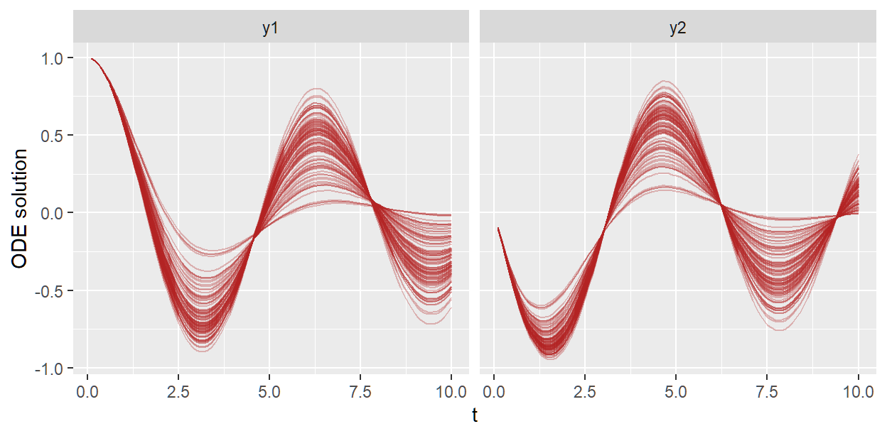
We can plot the distribution of ODE solutions like so
sho_fit_prior$plot_odesol_dist(include_y0 = TRUE)
#> plotting medians and 80% central intervals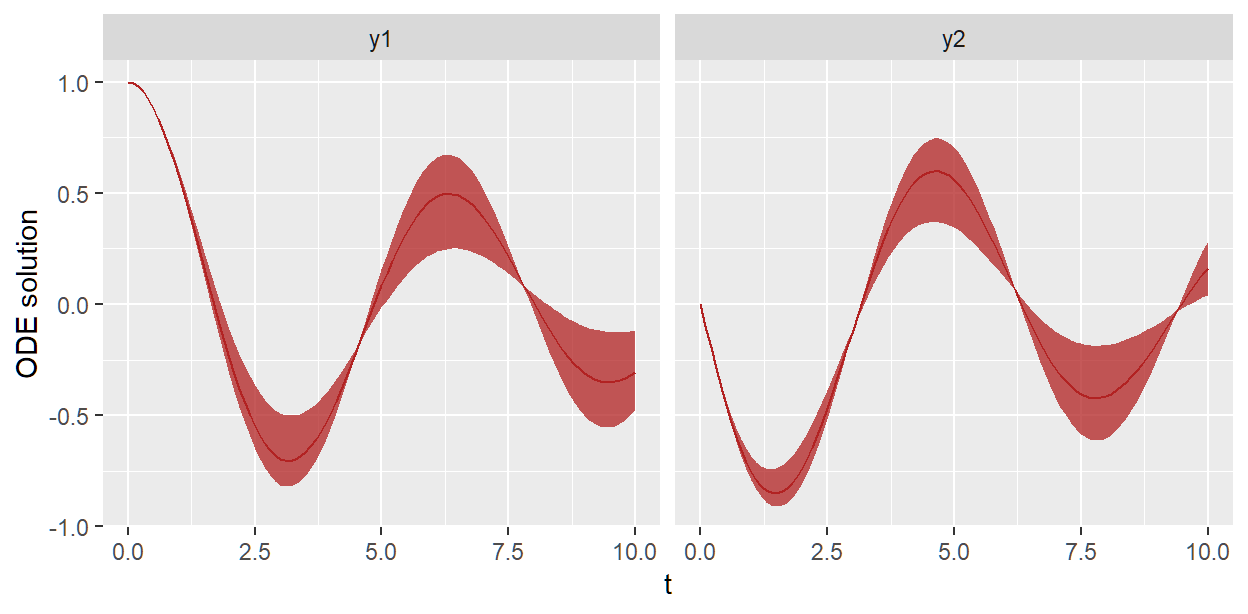
We can plot ODE solution using one draw like so
sho_fit_prior$plot_odesol(draw_inds = 45)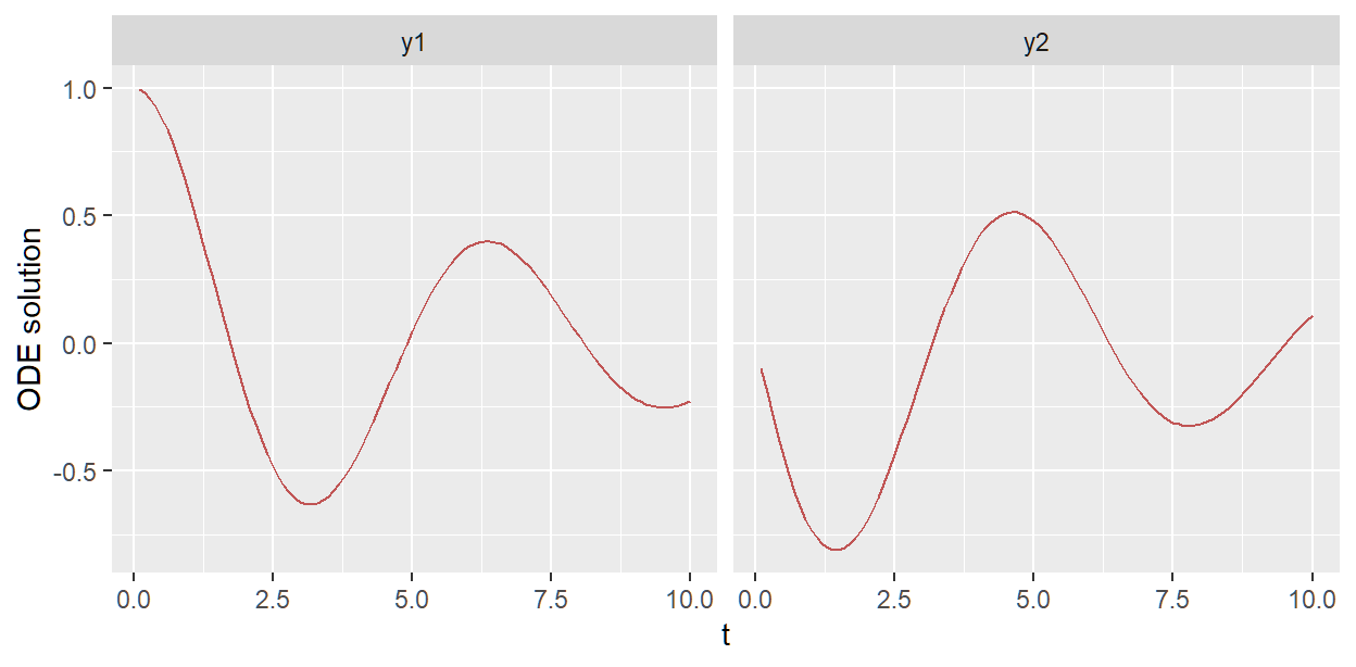
3 Using different ODE solvers
We generate quantities using a different solver and different output time points t. Possible solvers are rk45(),bdf(), adams(), ckrk(), midpoint(), and rk4(). Of these the first four are adaptive and built-in to Stan, where as the last two take a fixed number of steps and are written in Stan code.
gq_bdf <- sho_fit_prior$gqs(solver = bdf(tol = 1e-4), t = seq(0.5, 10, by = 0.5))
#> Running standalone generated quantities after 4 MCMC chains, 1 chain at a time ...
#>
#> Chain 1 finished in 0.0 seconds.
#> Chain 2 finished in 0.0 seconds.
#> Chain 3 finished in 0.0 seconds.
#> Chain 4 finished in 0.0 seconds.
#>
#> All 4 chains finished successfully.
#> Mean chain execution time: 0.0 seconds.
#> Total execution time: 0.5 seconds.
gq_mp <- sho_fit_prior$gqs(solver = midpoint(num_steps = 4), t = seq(0.5, 10, by = 0.5))
#> Running standalone generated quantities after 4 MCMC chains, 1 chain at a time ...
#>
#> Chain 1 finished in 0.0 seconds.
#> Chain 2 finished in 0.0 seconds.
#> Chain 3 finished in 0.0 seconds.
#> Chain 4 finished in 0.0 seconds.
#>
#> All 4 chains finished successfully.
#> Mean chain execution time: 0.0 seconds.
#> Total execution time: 0.5 seconds.We can again plot ODE solution using one draw like so
gq_bdf$plot_odesol(draw_inds = 45)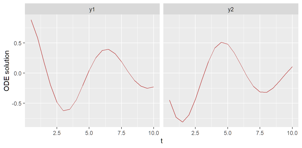
gq_mp$plot_odesol(draw_inds = 45)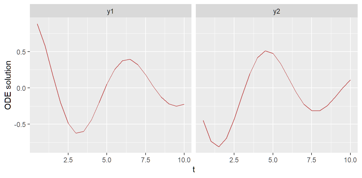
4 Defining a likelihood
Next we assume that we have some data vector y1_obs and define a likelihood function.
sho_loglik_body <- "
  real loglik = 0.0;
  for(n in 1:N) {
    loglik += normal_lpdf(y1_obs[n] | y_sol[n][1], sigma);
  }
  return(loglik);
"
In this function body, we can use the following variables without having to declare them or write Stan code that computes them:
- The ODE solution
y_sol. - Any variables that we give as
loglik_varsforode_model. - Any variables that are dimensions of
loglik_vars.
Here we define as loglik_vars a sigma which is a noise magnitude parameter, and the data y1_obs. Notice that we can also use the N variable in loglik_body, because it is a dimension (length) of y1_obs.
sigma <- stan_param(stan_var("sigma", lower = 0), prior = "normal(0, 2)")
y1_obs <- stan_vector("y1_obs", length = N)
The following code creates and compiles the posterior Stan model.
sho_post <- ode_model(N,
  odefun_vars = list(k),
  odefun_body = sho_fun_body,
  odefun_init = y0,
  loglik_vars = list(sigma, y1_obs),
  loglik_body = sho_loglik_body
)
print(sho_post)
#> An object of class OdeModel.
#>  * ODE dimension: int D;
#>  * Time points array dimension: int<lower=1> N;
#>  * Number of significant figures in csv files: 18
#>  * Has likelihood: TRUE
5 Sampling from posterior
Now if we have some data
y1_obs <- c(
  0.801, 0.391, 0.321, -0.826, -0.234, -0.663, -0.756, -0.717,
  -0.078, -0.083, 0.988, 0.878, 0.300, 0.307, 0.270, -0.464, -0.403,
  -0.295, -0.186, 0.158
)
t_obs <- seq(0.5, 10, by = 0.5)
and assume that initial state y0 = c(1, 0) is known, we can fit the model
sho_fit_post <- sho_post$sample(
  t0 = 0.0,
  t = t_obs,
  data = list(y0 = c(1, 0), D = 2, y1_obs = y1_obs),
  refresh = 0,
  solver = midpoint(2)
)
#> Running MCMC with 4 sequential chains...
#> Chain 1 Informational Message: The current Metropolis proposal is about to be rejected because of the following issue:
#> Chain 1 Exception: Exception: normal_lpdf: Location parameter is nan, but must be finite! (in '/var/folders/c6/f7ggr5956fs82hyz_p2qzsp00000gn/T/RtmpHS3GCA/model-152962319b414.stan', line 139, column 6 to column 60) (in '/var/folders/c6/f7ggr5956fs82hyz_p2qzsp00000gn/T/RtmpHS3GCA/model-152962319b414.stan', line 166, column 2 to column 62)
#> Chain 1 If this warning occurs sporadically, such as for highly constrained variable types like covariance matrices, then the sampler is fine,
#> Chain 1 but if this warning occurs often then your model may be either severely ill-conditioned or misspecified.
#> Chain 1
#> Chain 1 finished in 0.2 seconds.
#> Chain 2 Informational Message: The current Metropolis proposal is about to be rejected because of the following issue:
#> Chain 2 Exception: Exception: normal_lpdf: Location parameter is nan, but must be finite! (in '/var/folders/c6/f7ggr5956fs82hyz_p2qzsp00000gn/T/RtmpHS3GCA/model-152962319b414.stan', line 139, column 6 to column 60) (in '/var/folders/c6/f7ggr5956fs82hyz_p2qzsp00000gn/T/RtmpHS3GCA/model-152962319b414.stan', line 166, column 2 to column 62)
#> Chain 2 If this warning occurs sporadically, such as for highly constrained variable types like covariance matrices, then the sampler is fine,
#> Chain 2 but if this warning occurs often then your model may be either severely ill-conditioned or misspecified.
#> Chain 2
#> Chain 2 finished in 0.2 seconds.
#> Chain 3 Informational Message: The current Metropolis proposal is about to be rejected because of the following issue:
#> Chain 3 Exception: Exception: normal_lpdf: Location parameter is nan, but must be finite! (in '/var/folders/c6/f7ggr5956fs82hyz_p2qzsp00000gn/T/RtmpHS3GCA/model-152962319b414.stan', line 139, column 6 to column 60) (in '/var/folders/c6/f7ggr5956fs82hyz_p2qzsp00000gn/T/RtmpHS3GCA/model-152962319b414.stan', line 166, column 2 to column 62)
#> Chain 3 If this warning occurs sporadically, such as for highly constrained variable types like covariance matrices, then the sampler is fine,
#> Chain 3 but if this warning occurs often then your model may be either severely ill-conditioned or misspecified.
#> Chain 3
#> Chain 3 finished in 0.2 seconds.
#> Chain 4 Informational Message: The current Metropolis proposal is about to be rejected because of the following issue:
#> Chain 4 Exception: Exception: normal_lpdf: Location parameter is -inf, but must be finite! (in '/var/folders/c6/f7ggr5956fs82hyz_p2qzsp00000gn/T/RtmpHS3GCA/model-152962319b414.stan', line 139, column 6 to column 60) (in '/var/folders/c6/f7ggr5956fs82hyz_p2qzsp00000gn/T/RtmpHS3GCA/model-152962319b414.stan', line 166, column 2 to column 62)
#> Chain 4 If this warning occurs sporadically, such as for highly constrained variable types like covariance matrices, then the sampler is fine,
#> Chain 4 but if this warning occurs often then your model may be either severely ill-conditioned or misspecified.
#> Chain 4
#> Chain 4 finished in 0.2 seconds.
#>
#> All 4 chains finished successfully.
#> Mean chain execution time: 0.2 seconds.
#> Total execution time: 1.3 seconds.
We fit the posterior distribution of ODE solutions against the data
plt <- sho_fit_post$plot_odesol_dist()
#> plotting medians and 80% central intervals
df_data <- data.frame(t_obs, y1_obs, ydim = rep("y1", length(t_obs)))
colnames(df_data) <- c("t", "y", "ydim")
df_data$ydim <- as.factor(df_data$ydim)
plt <- plt + geom_point(data = df_data, aes(x = t, y = y), inherit.aes = FALSE)
plt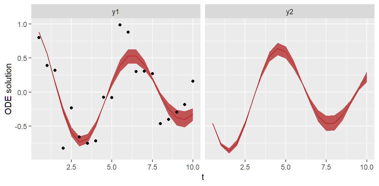
6 Reliability of ODE solver
Finally we can study whether the solver we used during MCMC (midpoint(2)) was accurate enough. This is done by solving the system using increasingly more numbers of steps in the solver, and studying different metrics computed using the ODE solutions and corresponding likelihood values.
solvers <- midpoint_list(c(4, 6, 8, 10, 12, 14, 16, 18))
rel <- sho_fit_post$reliability(solvers = solvers)
#> directory 'results' doesn't exist, creating it
#> Running GQ using MCMC-time configuration.
#> Running standalone generated quantities after 4 MCMC chains, 1 chain at a time ...
#>
#> Chain 1 finished in 0.0 seconds.
#> Chain 2 finished in 0.0 seconds.
#> Chain 3 finished in 0.0 seconds.
#> Chain 4 finished in 0.0 seconds.
#>
#> All 4 chains finished successfully.
#> Mean chain execution time: 0.0 seconds.
#> Total execution time: 0.5 seconds.
#> ==============================================================
#>  (1) Running GQ with: midpoint(num_steps=4)
#> Running standalone generated quantities after 4 MCMC chains, 1 chain at a time ...
#>
#> Chain 1 finished in 0.0 seconds.
#> Chain 2 finished in 0.0 seconds.
#> Chain 3 finished in 0.0 seconds.
#> Chain 4 finished in 0.0 seconds.
#>
#> All 4 chains finished successfully.
#> Mean chain execution time: 0.0 seconds.
#> Total execution time: 0.5 seconds.
#> Saving result object to results/odegq_1.rds
#> ==============================================================
#>  (2) Running GQ with: midpoint(num_steps=6)
#> Running standalone generated quantities after 4 MCMC chains, 1 chain at a time ...
#>
#> Chain 1 finished in 0.0 seconds.
#> Chain 2 finished in 0.0 seconds.
#> Chain 3 finished in 0.0 seconds.
#> Chain 4 finished in 0.0 seconds.
#>
#> All 4 chains finished successfully.
#> Mean chain execution time: 0.0 seconds.
#> Total execution time: 0.5 seconds.
#> Saving result object to results/odegq_2.rds
#> ==============================================================
#>  (3) Running GQ with: midpoint(num_steps=8)
#> Running standalone generated quantities after 4 MCMC chains, 1 chain at a time ...
#>
#> Chain 1 finished in 0.0 seconds.
#> Chain 2 finished in 0.0 seconds.
#> Chain 3 finished in 0.0 seconds.
#> Chain 4 finished in 0.0 seconds.
#>
#> All 4 chains finished successfully.
#> Mean chain execution time: 0.0 seconds.
#> Total execution time: 0.5 seconds.
#> Saving result object to results/odegq_3.rds
#> ==============================================================
#>  (4) Running GQ with: midpoint(num_steps=10)
#> Running standalone generated quantities after 4 MCMC chains, 1 chain at a time ...
#>
#> Chain 1 finished in 0.0 seconds.
#> Chain 2 finished in 0.0 seconds.
#> Chain 3 finished in 0.0 seconds.
#> Chain 4 finished in 0.0 seconds.
#>
#> All 4 chains finished successfully.
#> Mean chain execution time: 0.0 seconds.
#> Total execution time: 0.5 seconds.
#> Saving result object to results/odegq_4.rds
#> ==============================================================
#>  (5) Running GQ with: midpoint(num_steps=12)
#> Running standalone generated quantities after 4 MCMC chains, 1 chain at a time ...
#>
#> Chain 1 finished in 0.0 seconds.
#> Chain 2 finished in 0.0 seconds.
#> Chain 3 finished in 0.0 seconds.
#> Chain 4 finished in 0.0 seconds.
#>
#> All 4 chains finished successfully.
#> Mean chain execution time: 0.0 seconds.
#> Total execution time: 0.5 seconds.
#> Saving result object to results/odegq_5.rds
#> ==============================================================
#>  (6) Running GQ with: midpoint(num_steps=14)
#> Running standalone generated quantities after 4 MCMC chains, 1 chain at a time ...
#>
#> Chain 1 finished in 0.0 seconds.
#> Chain 2 finished in 0.0 seconds.
#> Chain 3 finished in 0.0 seconds.
#> Chain 4 finished in 0.0 seconds.
#>
#> All 4 chains finished successfully.
#> Mean chain execution time: 0.0 seconds.
#> Total execution time: 0.5 seconds.
#> Saving result object to results/odegq_6.rds
#> ==============================================================
#>  (7) Running GQ with: midpoint(num_steps=16)
#> Running standalone generated quantities after 4 MCMC chains, 1 chain at a time ...
#>
#> Chain 1 finished in 0.0 seconds.
#> Chain 2 finished in 0.0 seconds.
#> Chain 3 finished in 0.0 seconds.
#> Chain 4 finished in 0.0 seconds.
#>
#> All 4 chains finished successfully.
#> Mean chain execution time: 0.0 seconds.
#> Total execution time: 0.5 seconds.
#> Saving result object to results/odegq_7.rds
#> ==============================================================
#>  (8) Running GQ with: midpoint(num_steps=18)
#> Running standalone generated quantities after 4 MCMC chains, 1 chain at a time ...
#>
#> Chain 1 finished in 0.0 seconds.
#> Chain 2 finished in 0.0 seconds.
#> Chain 3 finished in 0.0 seconds.
#> Chain 4 finished in 0.0 seconds.
#>
#> All 4 chains finished successfully.
#> Mean chain execution time: 0.0 seconds.
#> Total execution time: 0.5 seconds.
#> Saving result object to results/odegq_8.rds
print(rel$metrics)
#>     pareto_k    n_eff     r_eff mad_loglik mad_odesol
#> 1 0.04886421 2575.384 0.6572188   1.230924 0.05165610
#> 2 0.06202465 2545.578 0.6561548   1.478181 0.06111844
#> 3 0.07737437 2533.872 0.6558465   1.566171 0.06441659
#> 4 0.07305680 2528.211 0.6557333   1.607148 0.06593929
#> 5 0.07093196 2525.093 0.6556848   1.629471 0.06676499
#> 6 0.06961408 2523.206 0.6556619   1.642952 0.06726222
#> 7 0.06871202 2521.980 0.6556503   1.651710 0.06758463
#> 8 0.06808765 2521.140 0.6556442   1.657718 0.06780550
unlink("results")
The mad_odesol and mad_loglik are the maximum absolute difference in the ODE solutions and log likelihood, respectively, over all MCMC draws. The former is denoted MAE in Timonen et. al (2023). Please refer to that paper in order to interpret the pareto_k column. Briefly we note that the Pareto-k values seem to be converging to a value smaller than 0.5, meaning that importance sampling is possible and we don’t need to run MCMC again.
7 References
- Timonen, J., Siccha, N., Bales, B., Lähdesmäki, H., & Vehtari, A. (2023). An importance sampling approach for reliable and efficient inference in Bayesian ordinary differential equation models. Stat, 12(1), e614. link